
A researcher has to explain a genetic result to someone who did not build the model. The software shows a precise score and a larger reference dataset. One practical question remains: does this comparison apply to the animals the person actually cares about?
A record count cannot answer that question on its own. The person needs to understand which animals were represented, what was measured, and where the result has been evaluated. Those details determine what the software can help them conclude.
Consider a dataset that doubles in size. An apparent relationship becomes stronger, until someone separates the data into its original groups. Within each group, the comparison points in the opposite direction. The calculation is reproducible; the aggregate needs more context to be useful.
Scientific software can make that context understandable. It can connect a result to its population, show the comparisons behind it, and explain where its applicability remains open. The engineering challenge is preserving those distinctions as data moves from the analyst's workspace into someone else's decision.
State which question the evidence is meant to answer
An observed frequency, a prediction, an estimate of genetic value, and a causal claim are different outputs.
A frequency describes a defined set of measured records. A prediction estimates an outcome for a target setting. An estimated genetic value depends on a specified model and population context. A causal claim asks what would happen under a change in an exposure or intervention, with additional assumptions about why the observed association arose.
Those differences should affect scope, validation, and presentation. A chart showing the fraction of tested animals with a reported outcome does not automatically estimate the outcome rate among all eligible animals. A model that predicts well within a particular family structure has not thereby established how it will perform in a new population.
The engineering team needs the intended question in language specific enough to test. Otherwise, a correct calculation can be presented as support for a stronger conclusion than the design permits.
Make the denominator visible
Scientific records often distinguish eligible subjects, measured subjects, records with an available outcome, and records excluded by a particular analysis. The distinctions matter when deciding what a proportion means.
Missing information can have several origins. A subject may never have been measured, a source may not supply a field, an import may be incomplete, or an outcome may not yet have occurred within the observation window. Treating these situations as the same numerical zero changes the question being answered.
A useful dataset description records the inclusion rules, observation window, measured counts, and known exclusions. It also retains the source's field definitions. Two columns with similar names may represent different measurement procedures or different levels of completeness.
These are product responsibilities as well as statistical ones. A user exporting a result should be able to understand its population and denominator without access to the private memory of the analyst who prepared it.
Work through a reversal caused by population mix
Consider the following constructed data. The labels describe no species, test, trait, or biological effect. The example demonstrates arithmetic only.
Synthetic counts by age group and marker status
Scroll to see all columns →
| Group | Marker present: records | Marker present: outcomes | Marker absent: records | Marker absent: outcomes |
|---|---|---|---|---|
| Younger | 20 records | 2 | 80 records | 16 |
| Older | 80 records | 64 | 20 records | 18 |
Within the younger group, the outcome proportions are 2/20, or 10%, for marker-present records and 16/80, or 20%, for marker-absent records. Within the older group, they are 64/80, or 80%, and 18/20, or 90%.
Now pool the groups. Marker-present records have 66 outcomes among 100 records, or 66%. Marker-absent records have 34 among 100, or 34%.
The direction reverses because the marker-present group contains a larger fraction of older records. The aggregate comparison uses different weights for the two age strata.
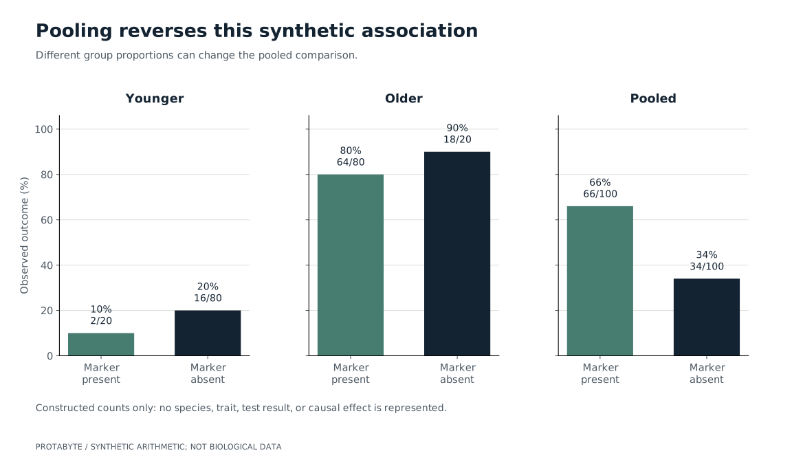
The pooled rate for a group is a weighted average of its subgroup rates. Changing the subgroup composition can change that average even when the within-subgroup rates are unchanged. A larger combined table can therefore make an association look stronger while changing which population the association describes.
Stratifying is not, by itself, a complete causal analysis. The example's lesson is narrower: the aggregate needs enough population context to be interpreted. A responsible interface should make the composition and comparison available for inspection.
Relatedness can be useful predictive information
It is tempting to summarize the validation problem as “related records are leakage.” Genetics requires a more careful account.
Genetic similarity and family relationships can be legitimate sources of predictive information. Work on whole-genome prediction examines how relationships between training and validation samples affect predictive performance. Beyond Missing Heritability includes a human study setting and discusses relatedness; its numerical results should not be transferred to an animal product.
The relevant engineering question is whether the validation setting resembles the intended use. If a system will predict within represented families with available historical information, a test that removes every such relationship may estimate a different task. If the system will be used for a new family or population, a random split that shares close relatives across training and evaluation may give an overly favorable picture of that intended use.
The task definition determines which comparison is informative. A validation design should state the target population and the relationship structure it is meant to represent.
Different splits answer different deployment questions
A random within-cohort split can help examine performance on records resembling the represented cohort. A family-held-out split addresses a different form of generalization. A later-cohort evaluation adds the effects of time, changing measurement practices, and evolving population composition. A population-held-out evaluation tests transfer to a particular excluded population.
These designs can be complementary. Their disagreement may reveal where a model's usefulness depends on the data available to it.
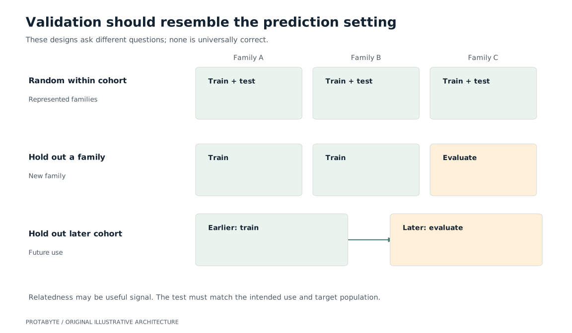
The product should retain the evaluation definition alongside any reported metric. That includes which records were available during fitting, which fields were known at prediction time, and which relationships the evaluation allowed.
Repeated measurements introduce another boundary. If several records concern the same subject, splitting records independently can put information from that subject on both sides of a comparison. Whether that is acceptable depends on the actual prediction task. Forecasting a later measurement for a known subject differs from predicting for a previously unseen subject.
A clear validation contract prevents those two tasks from sharing an ambiguous performance label.
Pooling reference data is a conditional modeling decision
Combining populations can increase the information available to estimate a model. It can also change population composition, the distribution of relevant features, and the relationship between markers and the quantities being predicted.
A cattle simulation study by Karaman and colleagues examined multiple pure breeds and admixed individuals under different modeling assumptions. Its findings include benefits from some combined-data approaches and limitations of simple pooling. The study supports a conditional account, rather than a universal rule that adding populations helps or harms prediction.
For an engineering team, this means the import pipeline and the evaluation pipeline need to agree on population definitions. A larger reference collection is an asset only in relation to a specified modeling task and target setting.
The team should also distinguish an operationally valid import from evidence that a model improved. A file can pass schema checks, preserve every source row, and integrate successfully while adding information that needs separate scientific evaluation.
Joined data brings uncertainty from the join
A scientific record assembled from several sources inherits the assumptions made during linkage. If an observation is assigned to the wrong subject, a model may see a relationship or sequence of events that does not exist.
Linkage uncertainty should therefore remain available to the analysis when it could affect the conclusion. A sensitivity check can examine an important result under plausible alternative assignments. That establishes how dependent the result is on the join, while leaving the identity question open.
This is consistent with methodological guidance that linkage errors can affect downstream analysis. Quality assessment in data linkage treats communication between the linkage and analytical stages as part of sound evaluation.
The useful product behavior is to expose a consequential assumption at the point where a person relies on it. An unresolved identity should not disappear merely because the next computation returns several decimal places.
Design the interface around the evidence actually available
A person opening a result needs a short answer to practical questions: who was represented, what was observed, and how closely the evaluation resembles their intended use. Population, observation coverage, source dates, and validation setting should travel with the result.
Start with a plain-language scope statement beside the result. Let the reader open the subgroup counts and evaluation details when they need to inspect them. A report should help an experienced reviewer check the analysis while giving another reader a clear account of what the result describes.
The interface can distinguish an observed absence from an unmeasured outcome, a supported within-population estimate from an untested transfer, and a calculation from an interpretation that still needs domain review.
A detail view can show the subgroup counts behind an aggregate, the cohort's inclusion rules, and which unresolved links or source gaps matter. Exported data should preserve those distinctions as well. Otherwise, a careful screen can become a misleading spreadsheet after the first handoff.
These choices also give the engineering team useful acceptance criteria. A reviewer should be able to reconstruct the denominator, explain the target population, and identify where the result's applicability has not been established.
Invest in the constraint that limits the next decision
The next valuable dataset may be larger. It may instead be better measured, better linked, or closer to the intended deployment population. A small representative evaluation can answer a question that a much larger convenience sample cannot settle.
A practical first milestone is to select one important product claim and specify its inference, population, information available at prediction time, and validation contract. Reconstruct the counts behind the current summary and test how they change under plausible source and cohort choices.
That gives technical leadership a concrete basis for the next investment. The objective is evidence strong enough for the decision the product is helping someone make, with the limits still visible when the data leaves the original analysis.
Protabyte builds scientific and data-intensive products that keep population context, source meaning, and interpretation connected. Talk with us about making a result useful to the person who has to rely on it.